
Motivation
One concept which is often discussed a lot in fields like mechanistic interpretability is a 'toolkit', a set of possible tools one can use to tackle some problem in understanding model internals.
For example, a lot of recent discussions talk about where sparse autoencoders fall into the mech interp toolkit (see Goodfire's Twitter thread[1]) with all their known issues such as L1 pressures discouraging interpretable features, and their poor performance compared to simpler linear probes (see Neel Nanda's work on this[2]). Despite all those discouraging signals, SAEs are still an important tool for any mech-interp researcher to have, and actually, we were able to use them to great effect to distill specific features into one of our newer models, Pipsqueak 3.
I think it's easy to theoretically understand where tools fall into the toolkit, but it's infinitely more beneficial to play with those tools and directly see their failures and successes in practice. For example, I never really understood the downsides of sparse autoencoders until I tried them against Parameter Decomposition for causal ablation experiments, and actually examined the feature activations and how different losses were changing results dramatically.
Post-trainer's Toolkit
One thing I am trying to develop for my own career is a 'post-trainer's toolkit', and I wanted to take some time after our most recent model release to really examine why whatever we threw at the wall worked. The main thing I've been meaning to examine is how I can add On-Policy Distillation to my toolkit. What role does it play amongst tools like Sequence Distillation (SFT) and GRPO? For a while, I was only looking at this from the perspective of Character.AI's use case, but I recently realized it's probably more insightful to take a step back and just examine it from a verifiable task's perspective.
The rest of this blog is my attempt at mapping out when, and more importantly how, OPD is useful on tasks such as mathematical reasoning. The findings in this blog are going to be largely disappointing, as they are well-grounded in theory that already exists from OPD's inception[3][4], but like I mentioned before, I think true understanding comes from actually implementing in practice rather than reading a couple of papers (on-policy learning??).
Brief understanding of OPD
It's probably a good idea to first revisit OPD.
Notation for the rest of this blog: is the student, is the teacher, is the prefix (the prompt plus everything generated so far) at position , and is the token sampled there.
On-policy distillation follows from the original REINFORCE[5] loss function as shown here:
where the advantage function is described as such:
Where is treated as a constant (stop-gradient). On-policy distillation changes to be the negative of a single-sample Monte Carlo estimate of the reverse KL divergence between the student's and teacher's policies. Ultimately, this just means replacing the formerly complex advantage function with the difference in log probability between a teacher and its student for a given token as such:
Writing out the gradients of the loss w.r.t. the pre-softmax activations provides some useful insight into what exactly OPD is doing.
The surrogate loss we examine for a single token is:
where denotes the stop-gradient operation. The gradients we care about are those with respect to the student's pre-softmax logits , where . Differentiating gives:
Writing out the derivative as a piecewise function to get rid of that indicator function, we get:
This gives us a fairly intuitive interpretation of OPD.
When the advantage is positive (where the teacher prefers a student-sampled token more than the student does), gradient descent increases the sampled token's logit while decreasing all other tokens' logits by a factor of the advantage and the tokens' current probabilities.
When the advantage is negative (where the teacher prefers a student-sampled token less than the student does), gradient descent will decrease that token's logit while pushing all other tokens towards a higher probability. Notably, because this scales w.r.t. the tokens' probabilities, this means the student's second and third choices get pushed higher than any other tokens do.
Collecting data
The first thing I wanted to do was just collect some data on verifiable tasks for OPD. I decided to do a sweep over a subset of a model family, and chose Qwen3[6] for this.
I took two teacher candidates (32B and 8B) and three student candidates (0.6B, 1.7B and 4B base). These models notably do not have thinking traces, as the thinking models of the same size were already distilled from the teachers.
For data, I used DeepMath-103k[7]. I had the teachers generate 32k traces total, filtering to ensure all 32k samples had validated correct solutions and stratified over difficulties 3-8. For the first phase, each teacher-student pair was trained on 24k samples of the rollouts, and evaluated against the MATH-500[8] dataset.
From there, for each model, I had each checkpoint do either 125 steps of OPD or 8k more samples of SFT (to ensure the same number of sequences used). This results in a graph we can analyze in more detail.
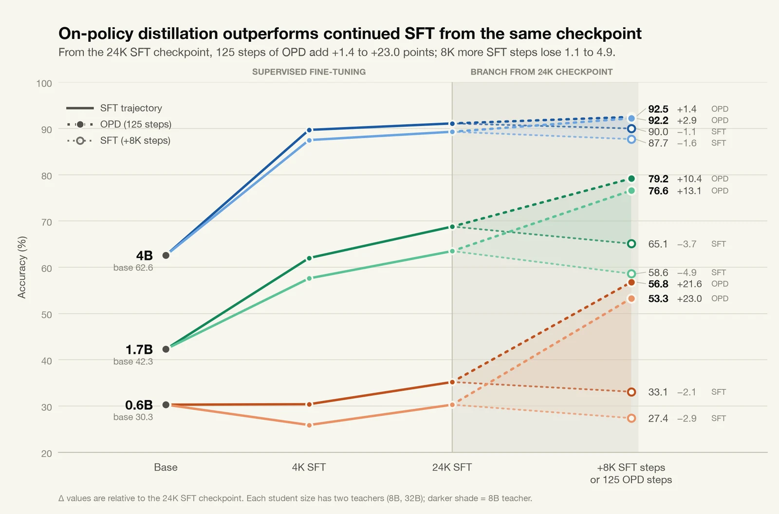
The results were far greater than I anticipated. There are some interesting things to note: on all models, the smaller 8B teacher outperformed the larger one in the SFT phase.
Secondly, the 8k additional fine-tuning resulted in worse performance in all cases. I attribute most of this to the model not having LR decay plus the optimizer states being reset to near 0. I ran this a couple of times to ensure this wasn't some fluke and double-checked the data quite a few times.
And lastly, the OPD performance was very significant. OPD led to massive gains on all models, which is especially impressive since SFT was nearly saturated when OPD started. One thing to note is I didn't try running SFT for a significantly longer time (simply because of compute budget issues), so I can't necessarily back up the prior claim that SFT would not continue increasing after a while. But regardless of that, the point was to check if OPD truly lived up to its hype, and that is definitely the case.
None of the above is shocking, nor should it be, given how OPD is now adopted by nearly every lab training a model, but it's fun to see the results for yourself. Furthermore, there really isn't a lot of literature that compares OPD to just continuing SFT for some reason; it largely only compares to other on-policy techniques. Part of that likely just has to do with the fact that on-policy training is significantly more expensive than SFT, and so it makes sense to just compare against equally compute-expensive methods.
But Why?
Now comes the part I actually cared about: why exactly are we getting these gains from OPD?
There are a couple of high-level ideas that I came to before which I think are worth investigating.
The first is what I'll call the 'capacity gap hypothesis'. In teacher-student distillation, we know there is a computational gap between the teacher and the student simply because of parameter size. It therefore should not be too hard to believe that in teacher traces, there are likely sections of compressed traces which a student would require more reasoning time to decompress.
To take a human example, whenever you first start doing LeetCode, there's a common pattern you learn that is quite useful to start. You typically jot out the whole naive solution, understand the time complexity of the solution, and then find efficiency gaps between approaches. But after a while of doing this, it just comes naturally to you, or you are able to quickly understand the time complexity of a potential naive solution just by thinking about it rather than writing anything down. When teaching a new person how to do LeetCode, you don't start from the latter trajectory, you start from the first. Perhaps something similar is happening during standard SFT. Large teachers are compressing information that small students simply don't have the computational capacity to decompress.
A second plausible hypothesis (to me) is what I'll call the 'entropy hypothesis'. This is something I largely hear as a potential reason for why OPD is useful, and it has to do with the reverse-KL nature of OPD. Reverse-KL encourages 'mode-seeking' behavior, and perhaps this mode-seeking-ness allows the student to be confident in a small set of strategies or just largely be less uncertain on longer scale trajectories.
The most obvious hypothesis would be that OPD derives updates to its policy w.r.t. the student's trajectories, not the teacher. But this is just an observation, and doesn't provide any insight into why this could be a good thing (at least I thought so before this set of experiments).
The next sections are my attempts to prove or disprove each of these hypotheses.
Examining the capacity gap hypothesis
The capacity gap hypothesis makes a few predictions, so let's empirically see what we get.
OPD students should write longer traces than SFT students after the 24k checkpoint. They don't. On MATH-500 problems that both students solve, they use roughly the same number of intermediate steps. Students already write at double the teacher's length, and OPD leaves that alone.
OPD's accuracy gains should come from problems the teacher compressed. If we stratify MATH-500 by the teacher's solution length on each problem, OPD's gain over SFT is flat across buckets. The terciles are 0.51, 0.71 and 0.99, and the gains are +12.0, +12.0 and +12.5. Same at 0.6B with an 8B teacher.
SFT students should do better on "uncompressed" traces, so the 8B teacher's advantage should come from its longer traces. To test this, I took 24k samples of DeepMath-103k, looked at the ratio of length between the 32B and 8B teachers' traces on each sample, and split them into quartiles. The bottom quartile is "compressed": the 32B trace is 2.2x shorter than the 8B's (medians 3.3k vs 7.3k tokens). The top quartile is "uncompressed": the 32B trace is 1.26x longer. A random sample of 6000 serves as a control. After running each pair 6 times on these samples, we get the following results:
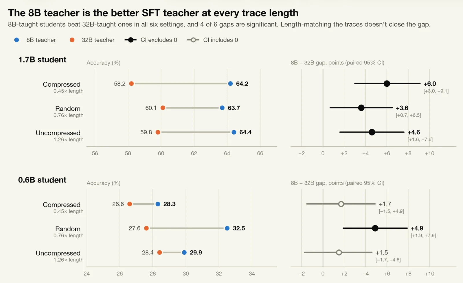
The 8B teacher largely keeps its SFT advantage regardless of length, suggesting the signal is something else like stylization, format, etc.
A smaller capacity gap should make a better teacher for SFT, but not matter for OPD. The first half holds, but the 8B teacher was better for OPD as well.
So, largely, the capacity gap hypothesis falls short. OPD isn't necessarily deriving its gains specifically from cases where the student is not able to decompress the teacher's reasoning.
Examining the entropy hypothesis
A commonly cited claim for the OPD gains has to do with the advantage forming (the negative of) an estimate of the reverse-KL between a teacher and a student. This should lead to 'mode-seeking' behavior from the student. If some large teacher has the ability to express multiple reasoning strategies where a student cannot, then the student faces little pressure to model both and instead can place a large amount of mass on only one of the modes. This contrasts with forward-KL, where the student is pressured to smear its mass over both modes, and can lead to a state of uncertainty. My next goal was to test if this is the true advantage of OPD over other approaches.
To understand this a bit better, we can revisit the advantage and its gradients. Let's take some student and some teacher . Suppose for a given token position , has the ability to express multiple valid possibilities with reasonable modes. As an extreme example, let's say:
Now, let's look at what happens when we use our standard reverse-KL approach. For reverse-KL, we sample from the student, so we expect to see token 99% of the time and token 1% of the time.
In the case of choosing token b, we would get the following gradient according to our previously defined derivative and advantage function:
Under gradient descent, this is a massive upward pressure driving token b towards a 50% probability. Looking at when token is sampled we can do the same calculation:
Since is the sampled token, its gradient is:
However, we also care about the gradient on token when is sampled, since this occurs 99% of the time:
So the expected update to is:
Therefore, we can expect very marginal gains on token b's probability, keeping token a as the dominating factor: "mode-seeking behavior". But what happens if we choose to sample from the teacher at the same prefix instead?
This is essentially what happens in ordinary cross-entropy training, where the teacher supplies the target tokens. We can express cross-entropy using the same surrogate loss as before, except with a constant advantage of 1:
Our gradients with respect to the pre-softmax logits now become:
Revisiting the same example:
When the teacher samples , the gradient on is:
When the teacher instead samples , the gradient on is:
Since both tokens are sampled with equal probability, the expected gradient becomes:
We expect a massive update to token b: 'mass-covering behavior'. Stepping back for a minute, what we are effectively doing in this approach is a strange hybrid of on-policy learning where we effectively reject the reverse-KL 'advantage'. At each iteration of a new problem, we sample a new student policy trajectory, and then for each token position, have the teacher sample what it expects the new token to be. From there, it's simple SFT. Obviously, this is super demanding to do, so we can run staler versions of this in reality, where we only get new traces after some number of updates.
When I was playing around with this idea as an attempt to either prove or disprove the entropy hypothesis, I eventually fed my reasoning into ChatGPT to see if this was valid at all. It turns out (of course) this is an already well-tested idea from 2011 called DAgger (Dataset Aggregation)[9]. It was originally proposed for imitation learning in settings like video games rather than language models, but I'm sure someone has already done this with LLMs, I'm just too lazy to check. This blog isn't supposed to present anything novel, just my own, hopefully understandable approach to investigating the value of OPD.
Results for the entropy hypothesis
For my DAgger-style runs, I started from the 24k SFT checkpoint for each student, and I ran 16 rounds of the following:
For each round, we sample 500 prompts from the 8,000-prompt training set without replacement. The current student writes one response per sample. The Qwen3-32B teacher is then fed the student trace, and for each token we record the teacher's next-token prediction at Qwen's ideal sampling temperature of 0.6. We discard the log probability and keep only the token. The student is then updated by plain cross-entropy: the input is the prompt plus the student's own response ids, the target at each response position is the teacher's chosen label.
Let's call the above approach "iterated DAgger". As an extreme version, I also made static runs, where there are no new rounds and we only use traces from the 24k SFT checkpoint.
For 0.6B, the SFT start was 28.6% and the OPD run was 53.6%. The static and iterated DAgger runs reached 50.1% and 50.0% respectively.
For 1.7B, the SFT start was 63.3% and the OPD run was 76.4%. The static and iterated DAgger runs reached 73.0% and 73.2% respectively.
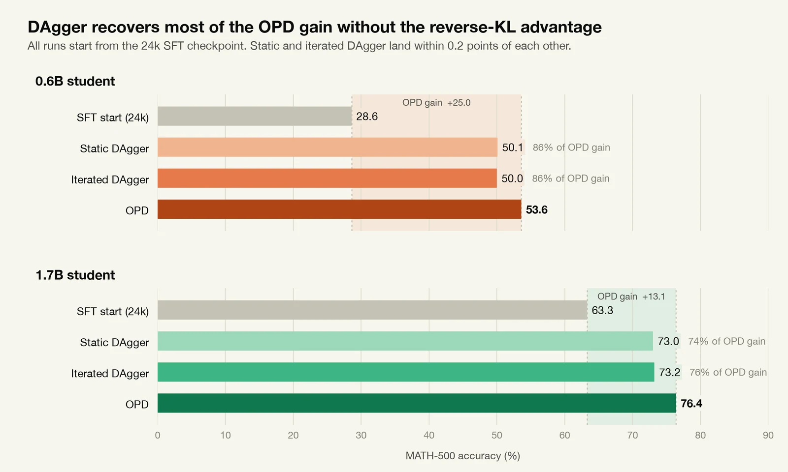
DAgger recovers most of the OPD gain, while, interestingly, not really requiring the iterated approach at all. That is something I will be examining in the future when I have more time.
In any case, we can sort of disprove the entropy hypothesis from this. Since we are seeing nearly equal gains from literally just sampling on student trajectories instead of the teacher's, while also having no "mode-seeking" pressure, it appears that most of the gain on OPD is coming from this phenomenon. This is exactly what I wanted to see out of this blog: instead of hand-wavy justifications of "use OPD because of reverse-KL mode-seeking pressure", we actually went inside to see that maybe this isn't the case, perhaps there is a better explanation for the gain, and this appears to be one possibility.
Now as it stands, this still isn't an explanation, it's just an observation about reverse KL. Luckily, since the technique ended up being so close to DAgger, we have a very convenient source for an explanation!
An explanation of DAgger's gains
Intuitively, the first thing that comes to mind for me for why this approach was more beneficial than SFT was the usefulness of the gradient information. During SFT, we are applying gradients to a policy on states it likely will never reach. Or in cleaner terms, at run time, the probability the student will reach a teacher's traces is exceedingly low. Now SFT does attempt to resolve this by literally performing that exact task, pushing student traces towards the teacher, but it's either incredibly slow or we expect some capacity restriction where there will be some gap that the student can simply not overcome.
In DAgger, we are already looking at plausible student states, and we are providing useful gradient information towards states we are more likely to see during runtime. Therefore, we help the model more when we provide gradient feedback on the more plausible student states than the teacher ones.
DAgger actually follows this reasoning fairly closely, though obviously with much better thought out formal reasoning. Let's say is the probability a student makes a mistake at every next token generation. Then, under behavioral cloning (plain imitation of the teacher's traces, which is what SFT does), when we are learning from a teacher we can examine specific scenarios to see the DAgger gain. Specifically, if we make the pessimistic assumption that from the moment makes a mistake, it will continue to make mistakes on every token until the trajectory ends at length , the error the student accumulates would be defined as:
So:
Or in other words, the error rate of the policy under behavioral cloning scales quadratically with the trace length. Under DAgger, we train on traces much closer to the student, including states where the student already made a mistake. Therefore, we can assume a more optimistic policy where the probability of an error is independent of prior errors in the trace, giving this:
Under DAgger (and some pretty lax assumptions), we should be able to effectively reduce the error rate by an entire order w.r.t. trace length.
Recap
So that sort of ends my week-long exploration of trying to understand 1) whether there are actual gains to be had with OPD and 2) where these gains are coming from. Writing out this blog was a pretty funny experience; I had all these prior assumptions about OPD that I completely forgot my original justification for in the midst of this process. I think I largely came out with what I wanted, which was an understanding of how effective OPD is on verifiable tasks and a general recipe for how I want to use OPD in my own toolbox.
From now on, I'll probably mostly use OPD as a last resort for gains on verifiable tasks. SFT is significantly more time-efficient (but not data-efficient), and one thing I didn't try with this approach was simply even more SFT data to see if there was any grokking effect.
When I observe SFT giving me diminishing returns, I'll turn to static DAgger and see what gains we can get from there, and likely iterated DAgger too. And likely a final OPD run just to see what remaining gains I can get.
One convenient part of using the above approaches first is that they support cross-tokenizer distillation well. It's something I didn't mention much before because I simply didn't have the compute or time to validate across model families as well, but in my experience cross-tokenizer OPD is particularly finicky. While it's easy to get pretty good coverage on most tokens using approaches like ALM[10] or simpleOPD, oftentimes nearly all advantages are negative, and in a lot of cases the teacher actually finds looping to be a more plausible behavior of the student than whatever potentially correct trajectory it's currently on.
It's pretty cool to add two new tools for the price of one (blog).
And lastly, just an overall note that feels fairly obvious in hindsight, it's probably a good idea to try techniques on verifiable tasks just to see what insights we can gain. This is really obvious, but since most of my experience comes from working on largely non-verifiable domains, it's something I'll definitely do in the future. Or at the very least try significantly harder to make some higher fidelity benchmarks, even if they don't correlate with the actual gain we want from a training run.
A series of causal ablations
This next section is sort of just spilling out data on things I tried in an attempt to understand, mechanically, exactly what is giving us gains during OPD. The past sections are all about this broader theoretical explanation, but I wanted to also literally see exactly what states were most important to our accuracy gains during training. I left this for last because I knew it wasn't going to be clean from the start; the signals are likely so intertwined that I can't say something like "numerical corrections by the teacher are the exclusive reason for OPD gains", but it was worth trying regardless.
First, let's look at corrections the teacher makes universally.
Teacher's "red pen"
The most common corrections are as follows:
Student wrote | Teacher wanted | Count |
|---|---|---|
|
| 358 |
|
| 244 |
|
| 243 |
|
| 211 |
|
| 183 |
|
| 168 |
|
| 160 |
|
| 159 |
|
| 152 |
|
| 146 |
|
| 140 |
|
| 135 |
Most of the corrections the teacher wants look to be at places we most expect. The student is either committing to a reasoning pattern the teacher does not like (the "therefore" to "wait" example), or doing the opposite ("?" to "." case). Numbers likely indicate arithmetic issues being common and needing to be corrected, and this pattern broadly extends for the rest of the list.
Also, from now on I am going to call pairs like ("therefore" to "wait") or ("?" to ".") pivot words. These signal points where the teacher wants the model to pivot to a different direction or towards certainty for its given trace.
Let's also look at the strongest objections, by looking at randomly drawn samples of corrections where the advantage was less than -2:
Context (...before) | Student → teacher | Adv | Read as |
|---|---|---|---|
...Democrats and Republicans as |
| -5.1 | wording |
...Instead of focusing on which balls go into which box, |
| -4.5 | wording |
...divisors of 24 larger than 1 are 2, 3, 4, 6, 8, 12, 24. |
| -9.5 | wording |
...−10 + 9 ≡ −1 |
| -2.7 | notation |
...set up the derivative |
| -6.3 | wording |
...= 4π/6 = 2π/3 |
| -3.0 | wording (confidence) |
...Then multiply 0.0059 × 1.32: |
| -5.1 | wording |
...90° clockwise: d + (z − d)e |
| -2.6 | substantive (sign of the rotation) |
...500 is 5^3 * 2^3, right? |
| -6.0 | substantive (500 = 5³·2²) |
...B includes all points on the boundary |
| -2.1 | substantive (about to misstate Pick's theorem) |
...(15 − 6.25) + 1 = 8. |
| -4.4 | substantive (garbled number) |
...tangent to each other and to two |
| -2.2 | substantive (wrong object) |
Interestingly, we do see a spread beyond just pivot words and numerical errors. A lot of these are stylization issues, like using "it" instead of "we" or the actual mod sign instead of the word.
Another thing I was curious to see is how the teacher annotates a trace after a critical error is made. Let's say a student makes a crucial mistake in a problem, like assuming a certain shape is symmetric and then wants to exploit that property for something like a geometric approach to an integral. Obviously we expect some large objection around the error, but would the teacher then harshly grade everything past the error as well, or would it allow the trace to continue using this symmetry argument and just assume the symmetry to see if the math plausibly continues from that assumption onwards? I expected the latter (which I feel like isn't optimal for learning), and it turns out we do see this. If we look at a subset of the words that resemble doubt (words like "but", "hmmm", "wait", "?", etc.) we see a bump close to the decisive error and then a fade back to the baseline. The "decisive error" is decided by pointing a 32B judge at student traces where the student was ultimately wrong and had a single point of error during the trace.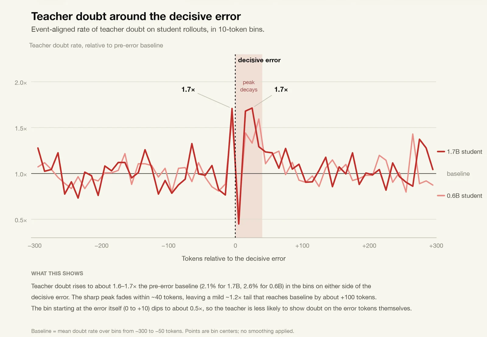
Finally, ablations
Based on the observations in the past section, I decided to run a series of runs where I ablate different tokens' advantages, either based on semantic understanding or advantage magnitude.
As each run took way too long as is, I decided to stop runs early at 25 steps and compare against full OPD at the 25th step as well.
A couple of notes on terminology, "veto" refers to negative advantages, states where the teacher does not prefer the student's token. "Hard vetoes" are vetoes below -2 in value. Confident states are states where the student is confident in the next token; I chose that to be under 0.8 nats. The results are below, and compared against full OPD and the SFT start.
"Wording" tokens refer to tokens that aren't pivots or numerical, so ideally represent stylization tokens mostly.
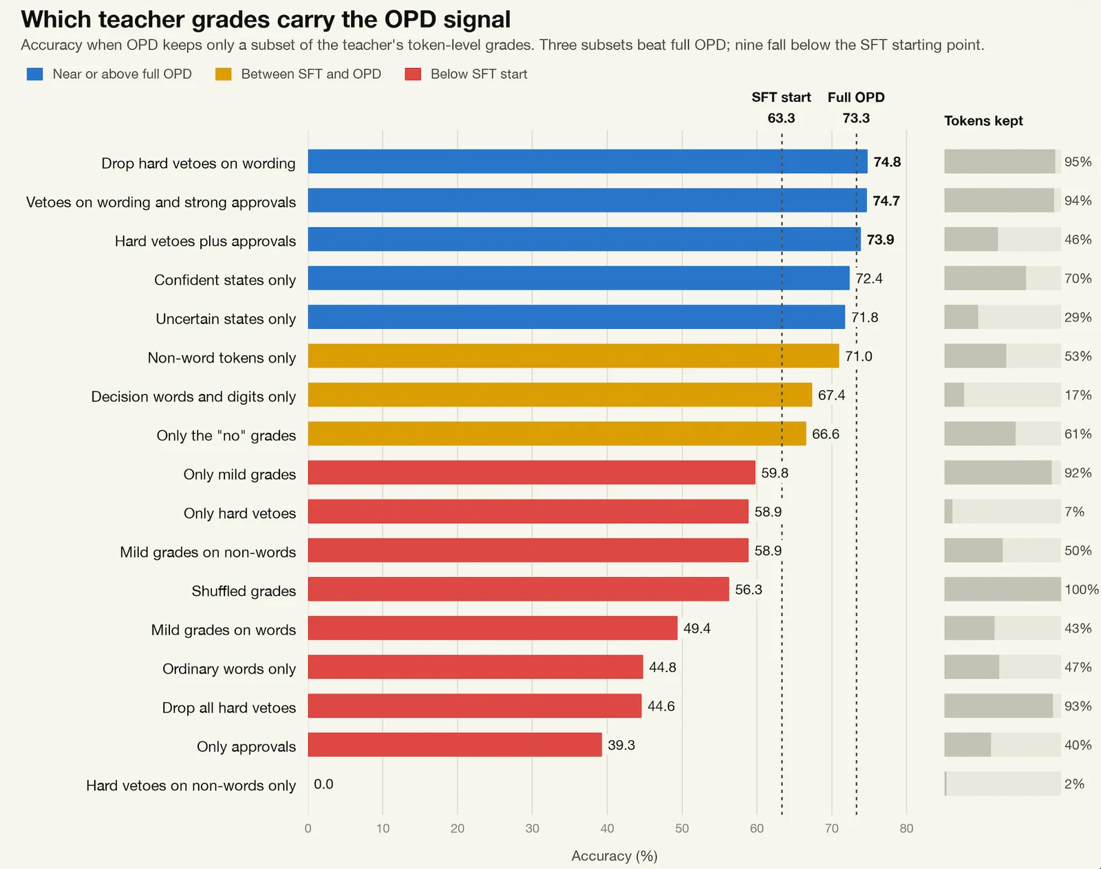
Unfortunately, there aren't any super cool results where we could isolate a specific signal for being responsible for most of the climb, but I did still manage to learn a bit from this. The first thing to note is we are able to remove some meaningful subset of tokens while fully recovering OPD gains, which can be seen with the "hard vetoes plus approvals" run. That run is particularly interesting because a majority of the signal from OPD skews negative (60/40 split), and to elaborate on that further, the exact splits for hard veto/mild veto/mild approval/strong approval over an average of 10 1.7B runs is 7.1%/53.9%/38.6%/0.44%.
Importantly, from our surrogate gradients we would predict that mild approvals have gradients extremely close to 0 and therefore hardly move the model. Coupled with the fact that strong approvals are exceedingly rare, how are we getting any gradient information from the positive signal? And if this is the case, we should expect that training on only hard vetoes recovers close to the same gain, yet it actually performs worse than SFT. What's going on?
We can first examine the hard vetoes only run. Actually looking at the traces, the model tends to collapse into looping significantly more, and thus most of the accuracy lost is on truncation (outside the 40,960 token window). Examining further, we can think about what a hard vetoes only run is actually doing. Hard vetoes land mostly on tail draws (47% of all gradient mass is hard vetoes on tokens that were not the student's first pick). And every veto is a push down on the token the student just drew. This combination leads to pushing the tail down repeatedly and the freed mass goes to the top pick, so the distribution sharpens everywhere, including on tokens that never received a gradient. The actual entropy of the model during the run supports this, going to 0.17 by step 10, and 0.01 to 0.03 at flat tokens, eventually looping.
The approvals are only 16% of the gradient mass as expected, but that mass is concentrated where it does the most work. Within approvals: tokens the student already gave 0.9 or more are 65% of approvals but 0.2% of approval mass. Mild approvals on tokens the student gave under 0.5 are 19% of approvals and carry 74% of the mass, strong approvals carrying the remaining 26%. A mild positive advantage of half a nat on a token drawn at p = 0.1 has gradient proportional to , so it moves that token's log-prob roughly as hard as a hard veto moves the top-pick token. This means we are pulling up hard on tail draws: the exact counter-force to the hard vetoes' push down. The entropy equilibrates at 0.38 instead of 0.17, so training keeps generating informative draws instead of looping.
This sort of hints further at issues with cross-tokenizer OPD, where the split between approvals and vetoes is bound to be significantly skewed, and likely why there are so many issues with looping when attempting it, though I haven't actually examined the entropy myself. Let's actually plot the entropy per run because it illustrates a fun picture of competing pressures. The following graph is the mean per-token entropy of the student at tokens it sampled from steps 1 to 25 (how long I ran each run for):
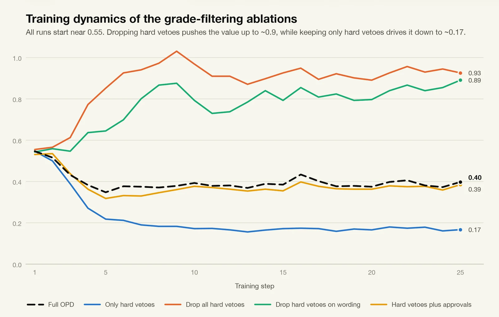
We can easily visualize the entropy pressures of different ablations which I think is a fairly cool graph for understanding. And this concludes the ablation section of this blog.
Recap 2.0
This is the final final end of the blog. The previous sections were actually more useful to me than I thought; they serve as a good starting point to understand where exactly OPD might be failing. For example, if I am observing looping at a significantly higher rate with OPD, I'm likely going to check the advantage distribution first and see if there is any potential benefit in advantage clipping (or something like binaryOPD instead).
I don't see why anyone would read this whole thing, but if you did, hopefully you came away with some new perspective or result on OPD.
IDK how to end this, bye.
References
- ^
Goodfire. Thread on sparse autoencoders, X. x.com/GoodfireAI/status/2104614372110909601
- ^
L. Smith, S. Rajamanoharan, A. Conmy, C. McDougall, T. Lieberum, J. Kramár, R. Shah, N. Nanda. “Negative Results for SAEs On Downstream Tasks and Deprioritising SAE Research.” LessWrong, 2025. greaterwrong.com/posts/4uXCAJNuPKtKBsi28
- ^
R. Agarwal, N. Vieillard, Y. Zhou, P. Stanczyk, S. Ramos, M. Geist, O. Bachem. “On-Policy Distillation of Language Models: Learning from Self-Generated Mistakes.” ICLR, 2024. arxiv.org/abs/2306.13649
- ^
K. Lu and Thinking Machines Lab. “On-Policy Distillation.” Thinking Machines Lab: Connectionism, 2025. thinkingmachines.ai/blog/on-policy-distillation
- ^
R. J. Williams. “Simple Statistical Gradient-Following Algorithms for Connectionist Reinforcement Learning.” Machine Learning, 8, 1992.
- ^
Qwen Team. “Qwen3 Technical Report.” 2025. arxiv.org/abs/2505.09388
- ^
Z. He et al. “DeepMath-103K: A Large-Scale, Challenging, Decontaminated, and Verifiable Mathematical Dataset for Advancing Reasoning.” 2025. arxiv.org/abs/2504.11456
- ^
H. Lightman et al. “Let's Verify Step by Step.” 2023 (source of the MATH-500 split). arxiv.org/abs/2305.20050
- ^
S. Ross, G. Gordon, J. A. Bagnell. “A Reduction of Imitation Learning and Structured Prediction to No-Regret Online Learning.” AISTATS, 2011. arxiv.org/abs/1011.0686
- ^
B. Minixhofer, I. Vulić, E. M. Ponti. “Universal Cross-Tokenizer Distillation via Approximate Likelihood Matching.” 2025. arxiv.org/abs/2503.20083